Mild Introduction to Modern Sequence Processing. Part 2: Recurrent Neural Networks Training

• 11 min
Experienced Software Engineer impassioned by AI, sharing my knowledge with you here
Examine the training process mechanics of Recurrent Neural Networks with a top ML specialist at Fively Andrew Oreshko as a continuation of the previous entry about RNN basics.
In our previous article, we learned the fundamental concepts of RNN and examined the core logic of forward pass. In this one, we are going to circle back to forward pass to review the formulas and to recollect the intuition on what the RNN is doing, and immediately after that, we turn our attention to the training process.

Many-to-One RNN: What Is It and How Does It Work
First, let’s examine in detail one of the variants of the RNN, a slightly simplified version of the model from the previous entry - many-to-one RNN. This one only outputs once the whole sequence (all the tokens of the sequence) is processed.

This architecture has multiple applications, like sentiment analysis, speech and handwriting recognition, machine translation, text and music generation, video analysis, time series forecasting, as well as dialogue systems and chatbots.
In the era of LLMs, one could argue that everything might be done using LLMs now, which is partially true, but examining how simpler models work gives a better insight into how it all evolved.
Overall, when one needs to map or represent a sequence to a single value, the many-to-one RNN can be useful, especially if you’re building your local model for your business, and don’t have enough resources to spin up/train/rent a powerful LLM. Also, it becomes easier to fine-tune your own model in case underlying data changes.
So, we’d like to advise to consider RNNs and their enhanced variants when a custom solution is developed (depending on a specific use case, of course).
There are also advanced variants of the basic RNN architecture, like LSTM and GRU. Those serve the same purpose as RNN but are highly better at capturing long-term dependencies, say long texts, due to their specific architecture bits. If interested, please take a good look at this well-recognized industry article.
We approach network training with a Backpropagation algorithm. It typically encompasses several steps that are:
- Forward Pass
- Loss calculation
- Backward Pass
- Weights update
The Backpropagation is run in a cycle until accurate enough predictions for the training data are reached – or the Loss is lowered to a reasonable extent.
For simplicity of telling, say we need to compose a model that learns to reply to “The Forest” with [0, 128, 0] (RGB for Green), to “The Sea” with [0, 0, 255] (RGB for Blue), to “The Fire” with[255, 165, 0] (RGB for Orange) effectively predicting a “color” of some natural event description. This is in fact a regression problem. All sequences have two tokens (a token would be a single word in our case). This is not strictly required of course but is done for simplicity as well, since if provided sequences were of various amounts of tokens then we’d need to apply techniques (which are out-of-context of the article), like padding to make them same-length token sequences which is required by RNN definition.
We can’t operate on raw strings hence those first need to be pre-processed.
“The Forest” could be encoded as [0, 1], “The Sea” - [0, 2], “The Fire” - [0,3]. In this regression setup, the output layer of the model will produce a 3-dimensional continuous vector representing the RGB color values – simply speaking an array of three.
As soon as the data is digitized, the model is able to start the Forward Pass. During that process, the data (the sequences) is fed to the net to produce outputs (y^t – predicted label from Figure 1) – 3-dim vectors just like the original labels – which are then used in Backward Pass - the main subject of the article that is outlined down below.
 Services Account
Forward Pass
Now, let’s look closer at the Forward Pass and how it works underneath.

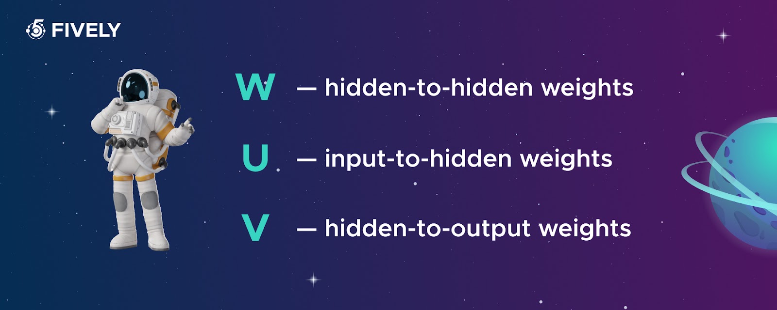
W, U, V are essentially parameter matrices which control how input data is transformed by the neural net to throw the predicted label at the end. If you recollect the simple linear function y = ax + b, the a, and b are similar concept – parameters that affect x (independent input data) to produce y (dependent label). The a affects the slope/gradient of the line, and b is the y-axis intercept which moves the line along the y-axis. You can imagine that you could possibly change a, and b to configure the equation to fit some set of data points (x and y coordinates).
This is a more-less dump recreation of what a neural network can do, and what factually our example model does – it builds some arbitrary function to fit input data (training data). Once we have the function built, we can get insight into what y could be, provided some value x – and we train the model to get its parameters/weights as accurately as we can to fit the training data and hopefully, the real-world data when it comes to testing/using it in prod environment.
h is a hidden state – the heart of RNN – it represents the model “knowledge through time (as I like to call it)”, as in RNN we need it to collect the context as we traverse the sequence. You could envision it like that: when you read some sentence, you’re trying to remember what you’ve read so far so that sentence still makes sense when you finish it. You most likely aren’t able to comprehend the idea of the message if you just see/remember one word. This “memory” is what a hidden state appears to be in the world of AI.
h0,1,2,..., t means hidden state value at a t time step.
Before Forward Pass comes into action, the weights and hidden state are somehow initialized: e.g. randomly or with zeros.
Forward Pass does just that: takes token sequences, one token at a time (called time step), multiples it by the U parameter, sums up with the product of the W parameter and current hidden state h, applies activation function over the result, and continues to do that, until inclusively the latest token (latest time step) is done and for which the latest h is calculated. Then we get the h times V parameter to get the predicted label.
Most transformations in the neural net are linear, like matrix multiplications that you can see on screenshots. Activation functions bring non-linearity to the table.
If there were no such functions incorporated that would apply non-linearity on top of those multiplications, no matter how many layers you’d put in, the model wouldn’t be able to learn these non-linear patterns, since the output of any layer was a linear transformation of its input – and that is why we use neural nets in the first place: learn complex non-linear patterns. An example would be finance, where lots of factors have an impact on stock prices, a quite popular application of ML.
The last step here is to calculate the error i.e. how far off the actual, or so-called ground truth, values that we want to see for the observations we used for training (the sequences) are spread out from the predicted values. The crucial thing here is that we need some accumulated representative number – the Loss.
The Loss can be calculated using a Loss Function, which typically varies from one neural nettype to the other, and from one application to the other. In our example as a baseline, we can leverage the Loss Function called MSE, mean squared error. The Loss function is a model hyperparameter so it is selected by the model developer.
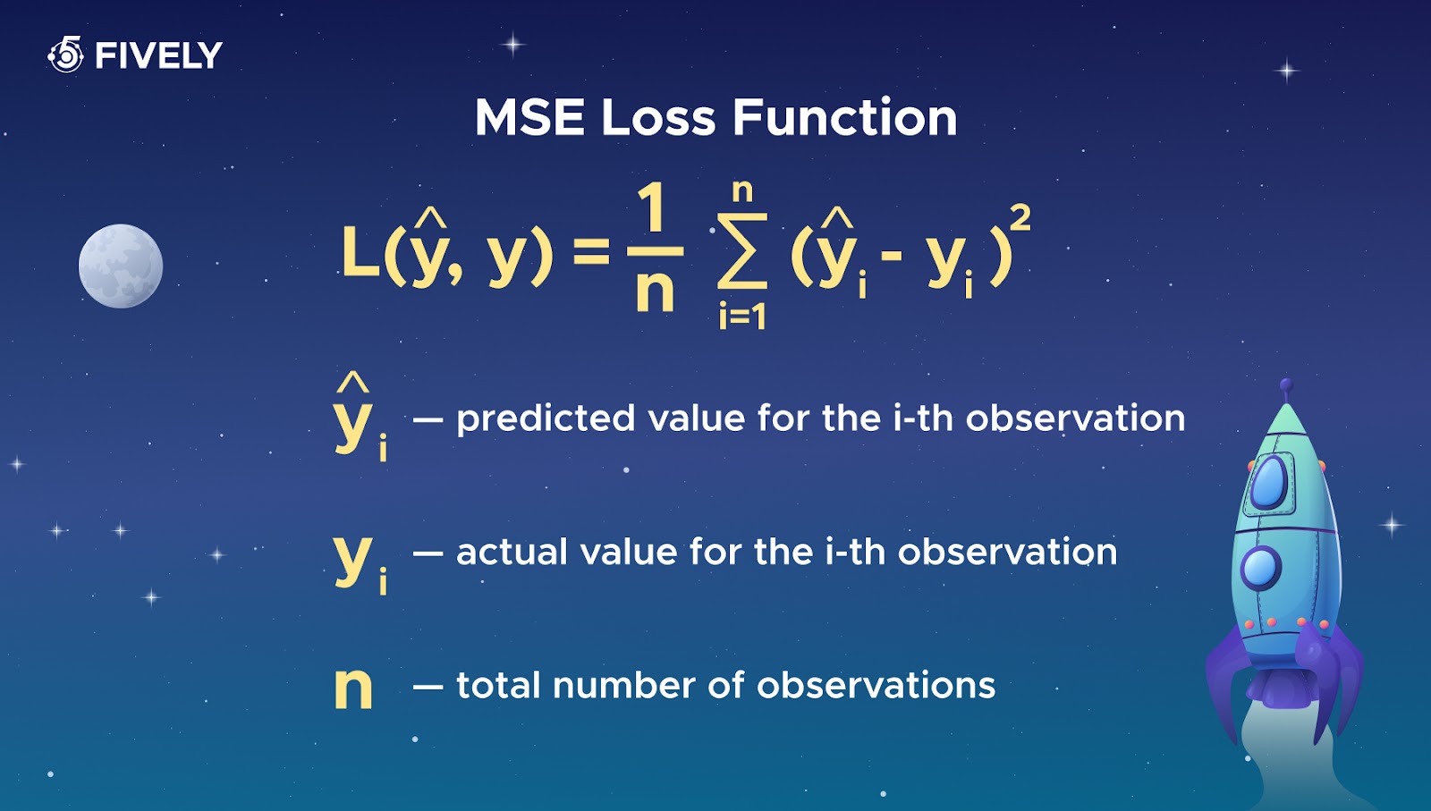
The result of the function above is the error that we need to propagate back through the net to tweak the model's parameters W, U, and V to lower the error.
Backward Pass
The Backward Pass is the essence and the most complex part of backpropagation. It operates on the result of loss, applying calculus and linear algebra, to deduce how to update weights to make the next Forward Pass output less wrong results.

Derivatives
Simply put, in calculus, a derivative shows how the function changes given its input change. Say, there is a function f(x) – its derivative at some arbitrary point x measures the slope of the tangent line to the function at that point. The nature of this slope line gives a sense of function behavior at that point x: If the derivative is positive, the function is increasing; if it’s negative, the function is decreasing. When the derivative is zero, the function has reached an extremum.
Speaking the real math language, the derivative of a function at some point is a limit of the ratio of the function differential to the argument differential. The differential is an infinitesimally small change of some variable. When the derivative of a function with a single argument is calculated, everything but the x in a function is naturally treated as constant(s). E.g., the derivative of the well-known function f(x) = x^2 (as well as f(x) = x^2 + 2) is f’(x) = 2x. The derivative of a constant value is 0.
Partial Derivatives
If a function depends on multiple arguments, a partial derivative is used to understand the function change concerning each individual argument. When the partial derivative is calculated, all args are treated as constants except for the arg, which the derivative is being calculated concerning.
Using derivatives, one gets to understand what to do to the argument in order to change the function value to the direction of choice. So it becomes more obvious now, why we need math/calculus in ML – using these terms we infer how to change the network parameters to actually lower down the Loss Function value, which reflects the overall error. This is what lies in the very foundation of any state-of-the-art ML system.
Backward Pass Logic
Our goal is to decrease the loss value. To do that, the W, U, and V need to be updated so that when the next forward pass round is executed, the loss lowers to some extent. The key idea is to calculate the gradient of loss. The gradient is a vector of the partial derivatives w.r.t to each argument, so we need to differentiate the loss function. The gradient just shows how the loss changes given all of those weights matrices change. The insight from calculus is that the gradient points in the direction where the loss increases the fastest. Naturally, we need to move in the direction of anti-gradient to decrease the loss value.
That’s why, as soon as we get the gradient, we become able to tweak those matrices as we need to.
Let’s check out formulas that allow us to do just that.
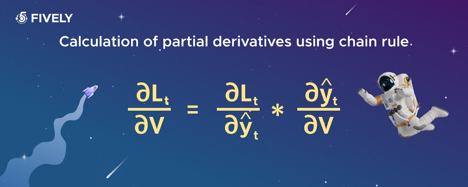
The one below is the simplest and depicts how to get gradient w.r.t to hidden-to-output weights. This one (and so are others) uses the chain rule method that enables the calculation of the derivative (when we talk derivative we imply the partial derivative) with respect to the argument that implicitly affects the differentiated function, by breaking the derivative down into the product of derivatives of the inner and outer functions: in the case of V, it is used to compute y^t, which in its turn is used to compute the loss as shown in Figure 4.
Hence, the chain - at first the derivative of loss w.r.t. to y^t is calculated, then the derivative of y^t w.r.t to, finally, V, is done. Ultimately, the product of these terms is taken, which results in a partial derivative of loss w.r.t to V – the first part of the loss gradient. This should more or less give an intuition of how this thing works: we’re basically talking gradient descent here. The same approach applies for W and U but is slightly modified.

The hidden-to-hidden derivative, too, is using the chain rule. We also work backward there, but since the W is affecting the hidden state all along the network, we need to walk through all the time steps to get the result, which is compactly shown above.
The actual tricky part here consists in the fact that the derivative of any, but the very first, time step hidden state w.r.t to the W is not just the derivative of h^t w.r.t to W itself – the W has an impact on the previous time step as well. As in, to get h^t, the W is needed alongside h^t-1, which likewise has been impacted by W. So, the h^t depends on W directly as well as indirectly, through h^t-1.
Exactly the same logic adapts to the computation of U, shown below.

Once we get the gradient at hand, the little part of the backpropagation remains to complete - weights update. We refine W, U, and V using the same technique: weight matrix = weight matrix - learning rate * weight matrix gradient. Subtract happens ‘cause we should move in the direction of anti-gradient. Learning rate is a critical network hyperparameter that controls how large a step you take towards minimizing the loss function. Without this coefficient involved, the gradient descent might take too large steps, and it typically results in very slow convergence (training time increases too much).
Recap
In this entry, we’ve walked you through the model training process, backpropagation, and its foundational steps. Also, we got a glimpse of calculus terms that form the basis of ML. But let’s move past the dull theories; the true way to learn any data-related aspect is through hands-on experience.
It’s time to create something genuinely working! In the next session, let’s build an advanced and extensively trained text generation RNN model using cloud GPU, and evaluate the outcomes. Stay tuned!
Services Account
Need Help With A Project?
Drop us a line, let’s arrange a discussion


